Traffic Sign Recognition
Classifying Traffic signs using a CNN
In this post I have explained my implementation of a Traffic Sign Classifier using a Convolutional Neural Network trained to classify German Traffic Signs. This project was of a part of Udacity’s Self-Driving Car Nanodegree Program. The complete code for the project can be found here.
Data Set Summary & Exploration
I used the Numpy library to calculate summary statistics of the German traffic signs data set:
- The size of training set is 34799.
- The size of the validation set is 12630.
- The size of test set is 12630.
- The shape of a traffic sign image is (32, 32, 3).
- The number of unique classes/labels in the data set is 43.
Exploratory visualization of the dataset
Here is an exploratory visualization of the data set. It is a histogram showing how the data is distributed by the labels in the training set.

We can observe that some classes such as Class 1 and Class 2 have a lot of data samples (about 2000 each) while some classes such as Class 0 and Class 19 have relatively much fewer data samples (about 200 each). This difference in the number of samples in a particular class may lead to the neural network learning more from the data belonging to the class with more number of samples the class than other classes that have relatively lower number of data samples. This makes the network biased towards a few classes during testing.
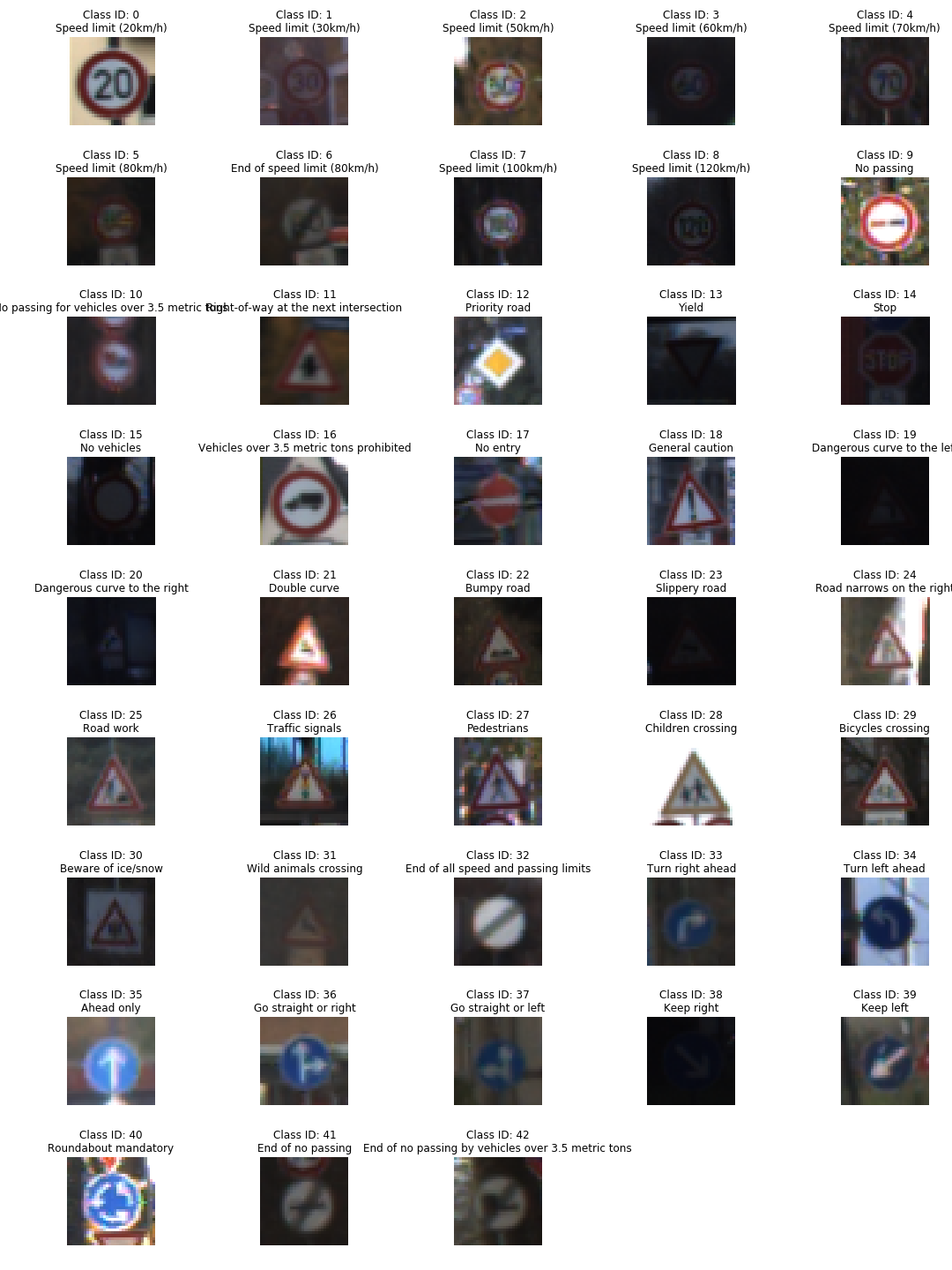
We can also observe sample images form all the classes to get some familiarity with the data along with their corresponding labels.
Data preprocessing
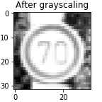
As a first step, I converted the images to grayscale because grayscaling removes clutter from an image. Since the problem includes only only classifying images, grayscaling allows the feature maps to concentrate only on the subject under interest. Also, grayscaling converts a 3-channel RGB image to a single channel image which reduces the computation complexity. Grayscaling was achieved by using the OpenCV’s cv2.cvtColor(image, cv2.COLOR_RGB2GRAY).
import cv2

# Convert to grayscale
def grayscale(image):
    gray = cv2.cvtColor(image, cv2.COLOR_RGB2GRAY)
    return np.reshape(gray, (32,32,1))
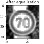
There were quite a few images that had low contrast and hence the signs were not clearly visible. This issue can be solved using histogram equalization which can be achieved using OpenCV’s cv2.equalizeHist(image). This basicaly enhances tthe contrast of the images and makes the traffic signs more clear. More information about histogram equalization can be found here. So, in the next step I applied histogram equalization on the grayscaled images.
# Histogram equalization to improve contrast
def histogram_equalize(image):
    equ = cv2.equalizeHist(image)
    return np.reshape(equ, (32,32,1))
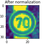
In the last step, I normalized the image data using the formula: (image/255) - 0.5. This step is necessary because normalization helps in making the neural network converge faster since the variation in data is restricted within a specific range (in this case between -0.5 and 0.5). An in-depth discussion on image data pre-processing techniques and their significance is provided in Stanford University’s CS231n course notes.
# Normalize images to improve convergence rate
def normalize(image):
    norm = image/255. - 0.5
    return np.reshape(norm, (32,32,1))

Model architecture and training
ConvNet architecture
I used a slightly modified version of the LeNet-5 architecture which is a simple 5 layer Convolutional Neural Network with 2 convolution layers, 2 fully connected layers, and a Softmax layer. The diagram below shows LeNet-5’s architecture.

I added a few dropout layers in between to reduce overfitting. My final model consisted of the following layers:
| Layer | Kernel Size | Number of filters | Stride | Description | Padding |
|---|---|---|---|---|---|
| Input | - | - | 32x32x1 pre-processed image | - | |
| Convolution | 5x5 | 6 | 1x1 | outputs 28x28x6 | Valid |
| RELU | - | - | - | Activation function | - |
| Max pooling | 2x2 | 6 | 2x2 | outputs 14x14x6 | Valid |
| Dropout | - | - | - | keep probability (0.7) | - |
| Convolution | 5x5 | 16 | 1x1 | outputs 10x10x16 | Valid |
| RELU | - | - | - | Activation function | - |
| Max pooling | 2x2 | 16 | 2x2 | outputs 5x5x16 | Valid |
| Dropout | - | - | - | keep probability (0.7) | - |
| Flattening | - | - | - | outputs 400 | - |
| Fully Connected | - | - | - | 400 input, 120 output | - |
| RELU | - | - | - | Activation function | - |
| Dropout | - | - | - | keep probability (0.7) | - |
| Fully Connected | - | - | - | 120 input, 84 output | - |
| RELU | - | - | - | Activation function | - |
| Dropout | - | - | - | keep probability (0.7) | - |
| Softmax | - | - | - | 84 input, 43 output | - |
Below is the code for building the network in TensorFlow:
import tensorflow as tf
from tensorflow.contrib.layers import flatten

def LeNet(x, keep_prob):
    # Arguments used for tf.truncated_normal, randomly defines variables for the weights and biases for each layer
    mu = 0
    sigma = 0.1

    # Layer 1: Convolutional. Input = 32x32x1. Output = 28x28x6.
    conv1_W = tf.Variable(tf.truncated_normal(shape=(5, 5, 1, 6), mean = mu, stddev = sigma))
    conv1_b = tf.Variable(tf.zeros(6))
    conv1   = tf.nn.conv2d(x, conv1_W, strides=[1, 1, 1, 1], padding='VALID', name = 'conv1') + conv1_b

    # Activation.
    conv1 = tf.nn.relu(conv1)

    # Pooling. Input = 28x28x6. Output = 14x14x6.
    conv1 = tf.nn.max_pool(conv1, ksize=[1, 2, 2, 1], strides=[1, 2, 2, 1], padding='VALID')

    # Dropout
    conv1 = tf.nn.dropout(conv1, keep_prob)

    # Layer 2: Convolutional. Output = 10x10x16.
    conv2_W = tf.Variable(tf.truncated_normal(shape=(5, 5, 6, 16), mean = mu, stddev = sigma))
    conv2_b = tf.Variable(tf.zeros(16))
    conv2   = tf.nn.conv2d(conv1, conv2_W, strides=[1, 1, 1, 1], padding='VALID', name = 'conv2') + conv2_b

    # Activation.
    conv2 = tf.nn.relu(conv2)

    # Pooling. Input = 10x10x16. Output = 5x5x16.
    conv2 = tf.nn.max_pool(conv2, ksize=[1, 2, 2, 1], strides=[1, 2, 2, 1], padding='VALID')

    # Dropout
    conv2 = tf.nn.dropout(conv2, keep_prob)

    # Flatten. Input = 5x5x16. Output = 400.
    fc0   = flatten(conv2)

    # Layer 3: Fully Connected. Input = 400. Output = 120.
    fc1_W = tf.Variable(tf.truncated_normal(shape=(400, 120), mean = mu, stddev = sigma))
    fc1_b = tf.Variable(tf.zeros(120))
    fc1   = tf.matmul(fc0, fc1_W) + fc1_b

    # Activation.
    fc1    = tf.nn.relu(fc1)

    # Dropout
    fc1 = tf.nn.dropout(fc1, keep_prob)

    # Layer 4: Fully Connected. Input = 120. Output = 84.
    fc2_W  = tf.Variable(tf.truncated_normal(shape=(120, 84), mean = mu, stddev = sigma))
    fc2_b  = tf.Variable(tf.zeros(84))
    fc2    = tf.matmul(fc1, fc2_W) + fc2_b

    # Activation.
    fc2    = tf.nn.relu(fc2)

    # Dropout
    fc2 = tf.nn.dropout(fc2, keep_prob)

    # Layer 5: Fully Connected. Input = 84. Output = 10.
    fc3_W  = tf.Variable(tf.truncated_normal(shape=(84, 43), mean = mu, stddev = sigma))
    fc3_b  = tf.Variable(tf.zeros(43))
    logits = tf.matmul(fc2, fc3_W) + fc3_b

    return logits
Training and hyperparameters
To train the model, I used the following hyperparameters:
- optimizer: Adam
- batch size: 128
- number of epochs: 50
- learning rate: 0.001
- mean (for weight initialization): 0
- stddev (for weight initialization): 0.1
# One hot encoding of labels
x = tf.placeholder(tf.float32, (None, 32, 32, 1))
y = tf.placeholder(tf.int32, (None))
one_hot_y = tf.one_hot(y, 43)

# define a new tensor for keep-prob (Dropout)
keep_prob = tf.placeholder(tf.float32, [])


# Model hyperparameters
EPOCHS = 50
BATCH_SIZE = 128
rate = 0.001

logits = LeNet(x, keep_prob)
cross_entropy = tf.nn.softmax_cross_entropy_with_logits(labels=one_hot_y, logits=logits)
loss_operation = tf.reduce_mean(cross_entropy)
optimizer = tf.train.AdamOptimizer(learning_rate = rate)
training_operation = optimizer.minimize(loss_operation)

correct_prediction = tf.equal(tf.argmax(logits, 1), tf.argmax(one_hot_y, 1))
accuracy_operation = tf.reduce_mean(tf.cast(correct_prediction, tf.float32))
saver = tf.train.Saver()


def evaluate(X_data, y_data):
    num_examples = len(X_data)
    total_accuracy = 0
    total_loss = 0
    sess = tf.get_default_session()
    for offset in range(0, num_examples, BATCH_SIZE):
        batch_x, batch_y = X_data[offset:offset+BATCH_SIZE], y_data[offset:offset+BATCH_SIZE]
        loss, accuracy = sess.run([loss_operation, accuracy_operation], feed_dict={x: batch_x, y: batch_y, keep_prob: 1.0})
        total_accuracy += (accuracy * len(batch_x))
        total_loss += (loss * len(batch_x))

    return total_loss/num_examples, total_accuracy / num_examples


from sklearn.utils import shuffle
with tf.Session() as sess:
    sess.run(tf.global_variables_initializer())
    num_examples = len(X_train)

    # initialize the training loss and training accuracy log arrays
    training_loss_log = []
    training_accuracy_log = []

    # initialize the validation loss and validation accuracy log arrays
    validation_loss_log = []
    validation_accuracy_log = []

    print("Training...")
    print()
    for i in range(EPOCHS):
        X_train_norm, y_train = shuffle(X_train_norm, y_train)
        for offset in range(0, num_examples, BATCH_SIZE):
            end = offset + BATCH_SIZE
            batch_x, batch_y = X_train_norm[offset:end], y_train[offset:end]
            sess.run(training_operation, feed_dict={x: batch_x, y: batch_y, keep_prob: 0.7})

        # training accuracy and loss
        training_loss, training_accuracy = evaluate(X_train_norm, y_train)
        training_loss_log.append(training_loss)
        training_accuracy_log.append(training_accuracy)

        # Validation accuracy and loss
        validation_loss, validation_accuracy = evaluate(X_validation_norm, y_validation)
        validation_loss_log.append(validation_loss)
        validation_accuracy_log.append(validation_accuracy)


        print("EPOCH {} ...".format(i+1))
        print("Training Accuracy = {:.3f}".format(training_accuracy))
        print("Validation Accuracy = {:.3f}".format(validation_accuracy))
        print("Training Loss = {:.3f}".format(training_loss))
        print("Validation Loss = {:.3f}".format(validation_loss))
        print()

    saver.save(sess, './lenet')
    print("Model saved")


## Test accuracy
with tf.Session() as sess:
    saver.restore(sess, tf.train.latest_checkpoint('.'))

    test_loss, test_accuracy = evaluate(X_test_norm, y_test)
    print("Test Accuracy = {:.3f}".format(test_accuracy))
Hyperparameter tuning
My final model results were:
- training set accuracy of 99.4%.
- validation set accuracy of 97.3%.
- test set accuracy of 94.5%.
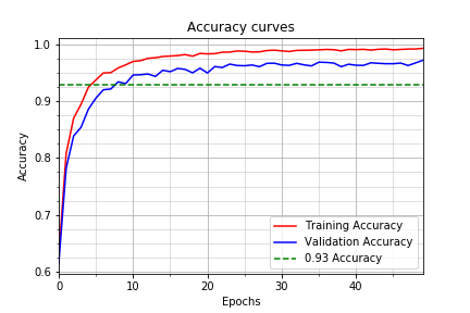
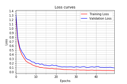
The following are my model’s accuracy and loss curves:
I chose an iterative approach to modify the Le-Net architecture to get the results:
What was the first architecture that was tried and why was it chosen?
I chose the LeNet-5 architecture as a starting point since it works well on hand-written digits.
What were some problems with the initial architecture?
There was a lot of overfitting with the initial architecture after feeding the network with the pre-processed data. The training accuracy was about 98% and the validation set accuracy was about 93%.
How was the architecture adjusted and why was it adjusted?
To reduce overfitting, I used 2 dropout layers after the 2 fully connected layers. I also used dropout layers after the max-pooling layers after experimentation since it reduced overfitting further. I experimented with different values for the keep probability and 0.7 seemed to provide the best validation accuracy on my architecture. Due to time constraints, I couldn’t experiment with different dropout rates for different layers which would have led to a more finely tuned network.
Which parameters were tuned? How were they adjusted and why?
I increased the number of epochs because the images were not as simple as handwritten digits with 10 classes. The traffic sign dataset contained 43 classes and the complexity of the images was also higher. To encode the information in this training set into the CNN required more nuber of epochs of training. After 10 epochs the validation set accuracy obtained was 93%, after 15 epochs it increased to 95%, and after 50 epochs it increased to 97.3%. This shows that the more number of epochs we train, the better the network learns the training data.
What are some of the important design choices and why were they chosen? For example, why might a convolution layer work well with this problem? How might a dropout layer help with creating a successful model?
Convolution layers are useful if the data contains regional similarity i.e. the arrangement of data points gives us useful insight about the spatial information contained in the daata. Images particularly contain useful spatial information which is an important feature. Convolution layers help in extracting these features.
Dropout turns off or sets the activation in some of the neurons in a layer to 0 randomly. This helps the network learn only the most important features in the images ignoring very minute details which might be noise and may change from image to image even belonging to the same class. This prevents the network from overfitting to the training data. It increases the accuracy on the validation set and hence the testing set. So, the network performs better on new images.
Testing our Model on new images
In general the images acquired from the web have a higher resolution than the images in the training dataset. These images have a lot of objects apart from just traffic signs. Since, my model does not work on newly seen images, I manually cropped the images so that it only contained the traffic sign. Some of the images collected from the ineternet have watermarks embedded on them which distorts the image and adds unwanted noise to them. Furthermore, my model only accepts inputs with an aspect ratio of 1:1 and of size 32x32. Hence, I resized them in order to fit them into my model which lead to a loss of detail in the images. These were a few issues that I encountered during data pre-processing.
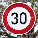
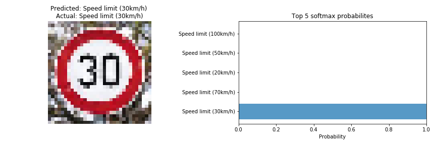
The first image should not be difficult for the model to classify because the characteristics (the number “30”) of the traffic sign are simple. But, it should also be kept in mind that there a lot of images in the training dataset that belong to the speed-limit class. So, the model might classify it incorrectly failing to distinguish it from other speed limit traffic signs.

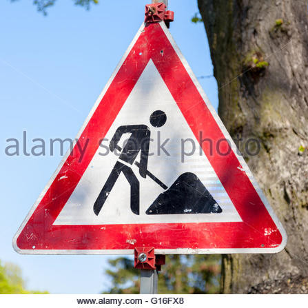
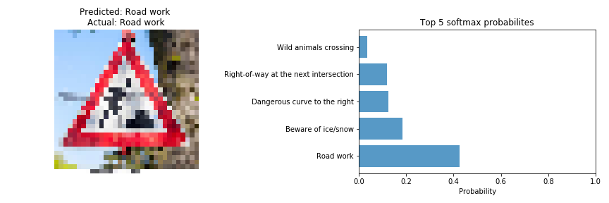
The second image might be challenging for the model to classify because it contains details. But, at the same time it is also very different from the rest of the class of images.
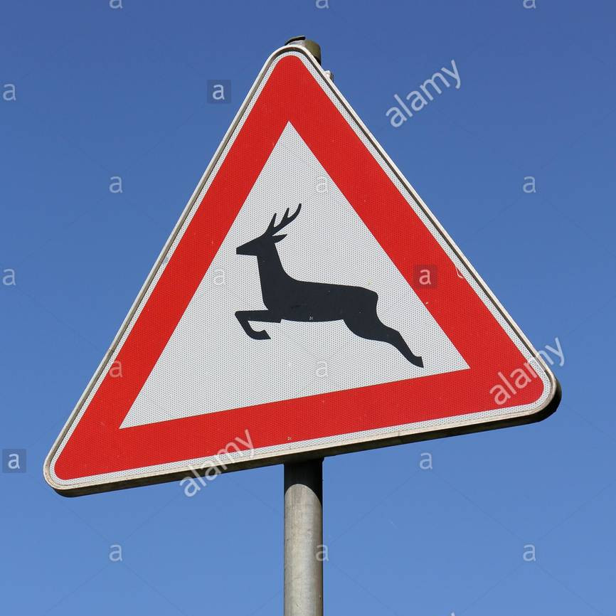
The third image should be difficult for the model to classify because the original image has details such as the deer’s antlers and legs which might be lost while down-sampling to 32x32. This might make it look similar to the “Turn left ahead” trafiic sign.
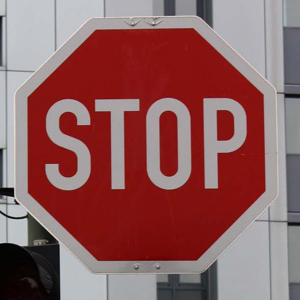
The fourth image should be easy for the model to classify since the characteristics (the “STOP” letters) of the traffic sign are very distinct from other traffic signs.
The fifth image might be challenging for the model to classify because it contains details. But, at the same time it is also very different from the rest of the class of images.
Performance on new images
Here are the results of the prediction:
| Image | Prediction |
|---|---|
| Speed limit (30km/h) | Speed limit (30km/h) |
| Slippery road | Slippery road |
| Wild animals crossing | Dangerous curve to the left |
| Stop | Stop |
| Road work | Road work |
The model was able to correctly guess 4 of these 5 traffic signs, which gives an accuracy of 80%. I actually downloaded 20 images from the internet and got correct prediction on 16 images which gives an overall accuracy of 80%. Although it is far lower than the accuracy on the test set, I feel that the major reason for the lower accuracy than the actual testing accuracy is that the images downloaded from the internet were originally of higher overall quality (resolution) than the training and testing images. On resizing the images to 32x32x3, some important pixels in traffic signs with detail e.g. road work, slippery road, wild animals crossing etc. were lost which might have led to lower accuracty on the internet images.
But, I was pretty confused as to why sometimes the model was not very certain while identifying speed limit signs. Since, the LeNet-5 network used was primarily used for digit recognition, I hoped that it would perform very well on speed limit signs which was not the case.
Looking into the Softmax probabilities
For the first image, the model is very certain that this is a 30 km/h speed limit sign (probability of 0.99), and the image does actually contain a 30 km/h speed limit sign. The top five soft max probabilities were
For the second image, the model is relatively certain that this is a Slippery road sign (probability of 0.89), and the image does contain a Slippery road sign. I did not expect the model to be so certain about this sign as after squeezing the image to a size of 32x32x3 some crucial pixels belonging to the road and the car in the image were lost that I felt were important in identifying the sign. The top five soft max probabilities were

For the third image, the model is certain that this is a Dangerous curve to the right sign (probability of 0.36), while the image actually contains a Wild animals crossing sign. I did not expect the model to be certain about this sign as after squeezing the image to a size of 32x32x3 some pixels belonging to the antlers of the deer were missing that I felt are crucial in identifying the sign. In fact, after reducing the size of the image the sign looks very similar to the class i.e. Dangerous curve to the left. But, the correct class for the image is the 2nd most probable sign as predicted by the model which is as expected. The top five soft max probabilities were

For the fourth image, the model is very certain that this is a Stop sign (probability of 0.99), and the image does actually contain a Stop sign. The top five soft max probabilities were

For the fifth image, the model is relatively certain that this is a Road work sign (probability of 0.77), and the image does contain a Road work sign. I did not expect the model to be so certain about this sign as after squeezing the image to a size of 32x32x3 some pixels belonging to the spade that the person in the image is holding were missing that I felt were crucial in identifying the sign. The top five soft max probabilities were
Visualizing the Neural Network
Visual output of the Feature maps
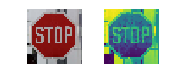
I took an image from the test images downloaded from the internet and fed it to the network.
The feature maps obtained in convolution layer 1 are
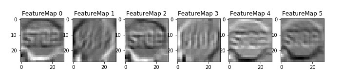
It can be observed that the feature maps of the first convolution layer encode the shape of the traffic sign and the edges of the image details, in this example the edges around the letters.
The feature maps obtained in convolution layer 2 are
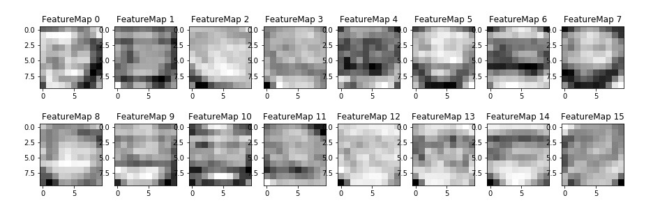
It seems that the feature maps of the second convolution layer encode more complex information and other minute details present in the traffic sign. It is difficult to comprehend what exactly the convolution filters are capturing in this layer.